Entry #2A: Designing Learning Problems
How Neural Networks Learn From Signals, Not Magic

I hit pause five minutes into Lecture 2 of CS230. Kian was already deep into a case study on day/night classification, but my notes were filling up with question marks. Not about the code—about the premise. The lecture assumed I already understood what 'learning' means to a neural network. I realized I needed to back up and answer that first.
This article makes that foundation explicit. We’ll synthesize the core theory from C1M1, CM1M2, and the recap of Lecture 2 into the mental model we need before the case studies make deep engineering sense.
1. The Core Loop: It’s Just a Function Getting Feedback
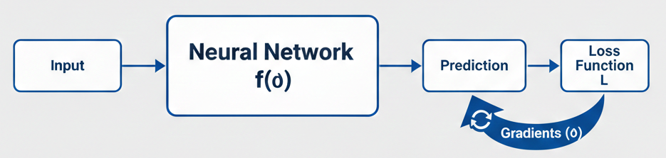
Strip away the biology metaphors. A neural network is, at its core, a parameterized function:
ŷ = f(x; θ)
xis our input (pixels, audio waves, words).θare the parameters (weights, biases)—the knobs to be tuned.ŷis the output (a prediction, a probability).
This function doesn't "know" anything. Learning begins only when we introduce a loss function: L(ŷ, y).
The loss answers one critical question: "How wrong was this prediction, and in what direction should we nudge the parameters to be less wrong next time?"
🧠 Mental Model: The network is a student. The loss function is the teacher. The gradients (calculated via backpropagation) are the specific, actionable feedback on the student’s work.
2. Data Design Is Our Information Ceiling
Lecture 2’s first case study—day vs. night classification—seems trivial. The key insight wasn't the model; it was a pre-training decision: image resolution.
The team didn't guess. They ran a human proxy test: "Can we tell if it's day or night at 32x32 pixels?"
If a human fails at a given resolution, a model trained via gradient descent will almost certainly fail too. This is a direct application of the principle from C1M1: the input defines the information ceiling.
🛠 Engineering Intuition: No loss function, no matter how clever, can recover a signal that isn't in the data. Our first design decision is ensuring the necessary signal survives preprocessing.
3. Labels Are Not "Truth." They Are a Design Interface.
In C1M2, labels (y) are presented as ground truth. In practice, they are a critical design interface. A label defines:
What the model should consider "correct."
What errors matter most.
What the gradients will emphasize.
This explains why label granularity is a leverage point. Compare two strategies for the "trigger word detection" problem:
Weak Interface: Label an entire 10-second clip as
1if "activate" is present.Strong Interface: Label each millisecond as
0(silence) or1(word spoken).
The data is identical. The gradient signal is radically different. The second approach provides precise, timely feedback, telling the model exactly where it needs to improve.
🧠 Mental Model: The loss function is the teacher, but labels write the lesson plan. A vague lesson plan creates confused gradients and slow learning.
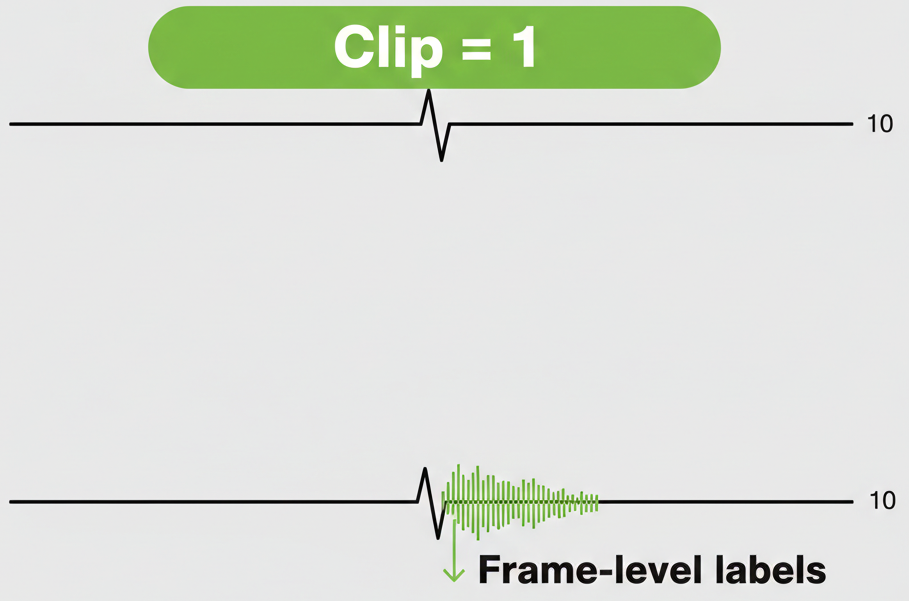
Two waveforms. Top: A single green bracket labeled "Clip = 1" over a 10-second clip with a tiny spike. Bottom: The same waveform with a dense, precise green highlight only over the spike, labeled "Frame-level labels". Visually contrast "vague" vs. "precise" feedback.
4. Gradients Are the Mechanism of Attention
From C1M2: Backpropagation computes how much each parameter (θ) contributed to the loss, generating a gradient for each. Parameters are then nudged in the direction that reduces the loss.
The crucial insight: A model learns what the gradients persistently emphasize.
Per-frame labels create strong gradients at specific moments, teaching precise localization.
A poorly designed label creates weak, noisy gradients everywhere, confusing the model.
Later, concepts like triplet loss work by designing a gradient signal that pulls similar data points together and pushes dissimilar ones apart.
🛠 Engineering Intuition: Debugging training often means asking: "What are my gradients actually telling the model to pay attention to?"
5. The "Two Files" Mental Model of Deployment
Lecture 2 offers a powerful, demystifying view of a trained system. A deployed model is just two files:
Architecture File: The code blueprint of
f(x; θ).Parameters File: The final, tuned values of
θ.
Everything termed "intelligence" is just numbers in File #2.
Training is the systematic process of using our data (x), our labels (y), and our loss (L) to find the set of numbers in File #2 that minimize L.
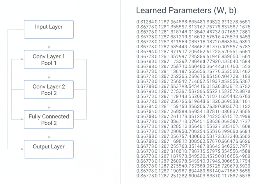
The left shows code architecture diagram (layers and connections), and the right shows a large matrix of numbers labeled as learned parameters.
Key Takeaway: The Signal is the Substance
Before we get lost in architectures, optimizers, or hyperparameters, we must answer the foundational question:
"What clear, learnable signal am I giving to the model, and what specific behavior does that signal reward?"
Supervised, self-supervised, and weakly supervised learning are merely different strategies for sourcing this signal. The engine—the gradient descent loop—remains the same.
This question is the true starting point of machine learning engineering. The case studies in Article 2B will show exactly how masters of the craft manipulate this signal to solve real problems.
References & Credits:
Concepts synthesized from Stanford CS230 Lecture 2


